Working with Basic Instrument Resonances Using Data and Techniques from J. Meyer
If you enjoy the technical side of things, please consider buying my book “Left-brain Lutherie” . Although no longer sold by StewMac, you can buy directly from me.
One of the most remarkable papers written about the acoustical properties of guitars is by J. Meyer in Issue #5 of the Journal of Guitar Acoustics. To me the paper is so fundamental and important that I have created a whole page to try to encourage others to read the paper in more detail and appreciate its significance.
There are two directions for understanding how some of the various resonances within the guitar and ukulele body work: 1) from within the building process by setting the top, back and body volume to various resonances and observing the outcome; 2) from observing resonance characteristics of a desirable finished instrument and trying to duplicate at least a portion of the response.
During the building process, the greatest possibilities for control over the final product exist, but the builder may or may not have a particular vision in mind. Conversely, when analyzing a finished (great) instrument, one knows that something wonderful has happened, but the manner in which it occurred may be extremely difficult to decipher.
DISCUSSION OVERVIEW: we’re first going to look at how the existing first resonances of the top plate, back plate and body volume of an ukulele/guitar interact with one another in the finished instrument. From this understanding we will then try to develop a rationale for approximately copying the sound properties of an existing instrument.
We cannot lose hope at this point. By utilizing Meyer’s work, we can truly understand more about the interactions of at least the first top resonance, first back resonance and air resonance with one another. This is a giant step. On this webpage we will try to show how Meyer’s work can be used for both building and retrospective analysis.
We begin with the simplest (although least musical) case: a guitar-shaped box with the soundhole in the usual place and the top, back and sides made extremely stiff. In such a system, there will be many resonances occurring within the body cavity as a function of the physical dimensions of the box. See Allen, American Lutherie, Issue #1 for additional details. In all likelihood the lowest resonance will be the Helmholz resonance; for a classical guitar of average dimensions it will have a value of 120-140 Hz. For a given: soundhole size & position, body shape and extremely stiff top, back and sides, this value is a constant and a fundamental measurement that must be made in order to go further with the type of calculations described by Meyer.
Rather than make the “concrete” ukulele/guitar, we can measure this resonance by suspending a small speaker in the finished guitar/ ukulele body and sweeping across a range of frequencies using a frequency generator and amplifier . Using a small microphone such as a Radio Shack lapel pin microphone attached to an oscilloscope or other amplifier, we can monitor either voltage or volume and determine when a peak occurs. Meyer labels the Helmholz resonance fO ; it is one of the three primary builder-controlled fundamental resonances that we will be studying (the other two being the first fundamental of the top and the first fundamental of the back). There may be several low frequency resonances associated with the body volume. The Helmholz resonance requires an opening to exist; if a measured resonance disappears when the soundhole is covered, then it is most likely the Helmholz resonance. Remembering that the top and back need to be stiff, it’s usually easiest to press the instrument body against thick pile carpeting (to muffle the back) while pushing down (gently but firmly) on the upper and lower bouts. After re-reading this, it sounds as though a second person would be needed to twiddle the frequency generator knobs and record data.
Measuring the Helmholz Frequency
Figure 1. Helmholz and Air Resonance Measurement 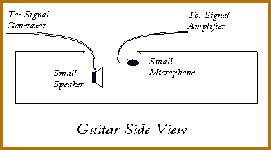
Here are the three main resonances which the builder can control during the building process:
fO = cavity resonance with stiff top, sides & back (Helmholtz)
fD = first top resonance with stiff sides & no back
fB = first back resonance with stiff sides & no top
Here are the resonances which result from interactions of the above three for the first two plots:
f ‘1 = cavity resonance with flexible top, stiff sides & back (air resonance)
f ‘2 = first top resonance with stiff sides & back
To obtain the following plots from the Meyer article, I hand-picked the data (very tiresome), re-plotted it and ran best-fit regressions on it to determine the equations associated with each plot. For some reason, Meyer did not choose to run these regressions or if he did, did not put them in the article.
Meyer Plots – Part 1
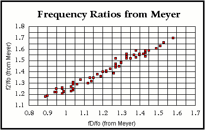
Figure 2. Meyer Plots — Plot 1 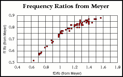
f ‘1/f O = – 0.42 * [f D/fO]2 + 1.30 * [ f D/fO] – 0.13 (1)
r2 = 0.98
I suppose the first thing that confused me about this type of plot (not being mathematically adept) was that both of the variables (f D and f ‘1) were divided by fO. In fact, it turns out to be a fairly common way of looking at data. It is a normalizing device. That is, if you were working with a range of instrument sizes, then you would have a range of Helmholz, top and back resonances simply because of differences in instrument size. Yet the relationships among the measured properties might be the same for all the different sizes. If we divide the data collected for a given instrument by its Helmholz resonance, we will be able to utilize the work already done by Meyer for classical guitar sized instruments because we have normalized the other resonances for our instrument relative to Meyer’s work.
So let’s look at the first plot. If f D is equal to fO, then f ‘1 is about 75% of its former value. I’m calling the altered value of the Helmholz resonance, the air resonance. The air resonance differs from the Helmholz resonance because the top, and/or back and/or sides are flexible rather than fixed. The implication of this is that the air resonance will always be lower than the Helmholz resonance because the surfaces of the cavity are more flexible (offer less resistance). As the top resonance, f D increases relative to the Helmholz resonance fO, the system behaves more and more like the “concrete guitar” and there is less of a difference between the Helmholz and air resonances. Since frequency is proportional to stiffness (in the absence of mass added for the purpose of lowering frequency), there will clearly be a point at which a given top frequency f D will be too low to provide sufficient mechanical stiffness to keep the top from deforming. I recommend that the reader also study the mechanical compliance webpage on this site for further understanding of this measurement process.
Meyer Plots–Part 2
f ‘2/f O = 0.77 * [ f D/fO] + 0.48 (2)
r2 = 0.97
The second plot shows a similar trend but now relating the altered top resonance f ‘2 rather than the air resonance f ‘1. When the top resonance f D equals the Helmholz resonance f O the top resonance increases by 25%. This increase occurs because the air trapped within the body of the instrument offers greater resistance to the vibration of the top. Remember that we are still in the relatively simple case of a stiff back and sides (although for some builders, this is actually the normal case).
For me there are several immediate take-home messages behind these two plots:
First, if you measure a body resonance and top plate first fundamental on a completed instrument, it is essentially guaranteed that these values will not equal the Helmholz resonance nor the value of the top plate first fundamental when the top is only attached to the sides and no back is on the instrument.
Second, there is a rational relationship among the changes which occur.
If we now put a back on the instrument with a range of stiffness values, we observe the trends in Figures Meyer 3 and Meyer 4. Here are the remainder of the main resonances which we can measure in the finished instrument:
f1 = cavity resonance with flexible top & back, but stiff sides ( final air resonance)
f2 = first top resonance with flexible back, but stiff sides (final top plate first resonance)
Meyer Plots–Part 3
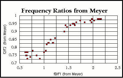
f 2/f ‘2 = – 0.214 * [ f B/f ‘1]3 + 0.84 * [ f B/f ‘1]2 -0.82 * [ f B/f ‘1] + 0.99 (3)
r2 = 0.97
In the above plot, we can see that at low values of the ratio of the first back plate resonance f B to the air resonance of the stiff-backed body f ‘1, the first top plate resonance f 2 for a flexible backed instrument is lower than the first top resonance f ‘2 for a stiff backed instrument. This is reasonable because a flexible back will constrain the air volume within the body less than a stiff back. In turn, a less constrained air volume will “push back” less against the top. As the frequency of the first back resonance f B increases, it becomes more and more like the stiff backed case and the ratio of the two different first top plate resonances approaches unity.
Meyer Plots–Part 4
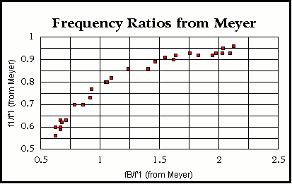
f 1/f ‘1 = – 0.217 * [ f B/f ‘1]2 + 0.82 * [ f B/f ‘1] + 0.16 (4)
r2 = 0.98
In the final plot, Meyer Plot 4, we can see that at low values of the ratio of the first back plate resonance f B to the air resonance of the stiff-backed body f ‘1, the air resonance f 1 for a flexible backed instrument is lower than the air resonance f ‘1 for a stiff backed instrument. This is reasonable because a flexible back will constrain the air volume within the body less than a stiff back. In turn, a less constrained air volume will have a lower resonant frequency. As the frequency of the first back resonance f B increases, it becomes more and more like the stiff backed case and the ratio of the two different air resonances approaches unity.
The figure below summarizes all of the variables discussed thus far in a descriptive format. The heavy lines represent thick fronts, backs or sides which do not have frequency measurements associated with them.
Figure 6. Meyer Variables as described in the text above: from left to right – 1. flexible front or back attached to stiff sides; 2. all sides stiff; 3. front flexible, back and sides stiff; 4. front and back flexible, sides stiff. 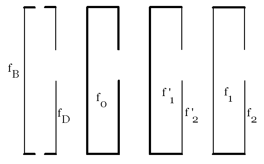 There is a simple test for determining how involved the back resonance is relative to the Helmholz and first top resonances. Hold the body of the instrument slightly away from your own body and gently tap against the bridge or where the bridge will be in the finished instrument. Now press the back of the instrument firmly against your own body (being careful not to scar the finish with buttons, etc.) and tap in the same place again. If the notes are essentially the same, then your instrument is very stiff backed. The greater the difference in the two tap tones, the more the back is involved with the other resonances.
After the Model…
Part 1 — Forward Modeling — Trying to create an instrument with a particular set of final resonance ratios
If you’ve read the work of Graham Caldersmith on guitars and Carleen Hutchins on violins, you probably know that making the first top plate resonance about an octave higher than the air resonance and a semitone above or below the back plate first resonance is a desirable feature in an instrument. But, gee…where to begin? Well, if you’ve chosen a particular shape, soundhole size and position, then the Helmholz resonance f0 is a fixed number. What you control is fD and fB as a result of their thickness and your choice of bracing and mechanical compliance. But the interaction of fD and fB with f0 will alter all three values. Further, fD is constrained somewhat because of the earlier mentioned relationship between mechanical compliance (to insure the physical integrity of the top) and string tension. Let’s now create a spreadsheet using Meyer’s formulae so that we can play with various combinations of our three builder’s parameters to achieve desirable player’s parameters. The name of the spreadsheet is MEYERCALCFWD.xls and is an Excel spreadsheet.
MEYERCALCFWD (to download double-click or option-click)
The two tables below show sample calculations done by the spreadsheet for a guitar. In principle, the calculations should work for any guitar family instrument, soprano ukulele through bass acoustic guitar. The three user changeable variables are f0, fD and fB in columns 2, 3 and 7 of the spreadsheet and are highlighted in light blue. In the case shown below, I have used an arbitrary but believable Helmholz resonance of 130 Hz for a classical guitar. I then initially put in a value of 200 Hz for fD and an incremental range of resonances for fB which bounded fD. I then went back and gently fiddled with the individual values of fD until a ratio of 2.00 for f2/f1 was reached. It is important to remember that this spreadsheet is simply a tool for general direction guidance. The actual precision of the calculations is probably in the order of 10-15%.
So what shows up in the spreadsheet? As predicted, the Helmholz ratio, f0, steadily decreases as first a flexible top and then a flexible back are added to the once rigid guitar body (for guitar #1: 130 –> 114 –> 102 Hz ). Interestingly, the top plate first resonance initially increases because of the resistance of the air cavity and then decreases as a flexible back is added (for guitar #1: 207 –> 222 –> 205 Hz ). If we wish to pursue our original goal of trying to have a back resonance a semitone above the top resonance, then assuming that both front and back resonances change in parallel, guitar #5 would be close judging from the fB/fD ratio. For the back to be a semitone below the top resonance, somewhere between guitar #2 and guitar #3 might be appropriate.
Table 1. First Half of MEYERCALCFWD.xls Spreadsheet Sample Calculations 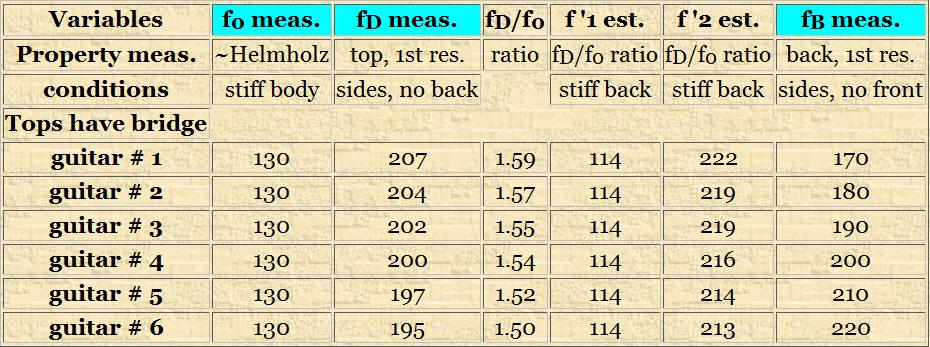
Table 2. Second Half of MEYERCALCFWD.xls Spreadsheet Sample Calculations 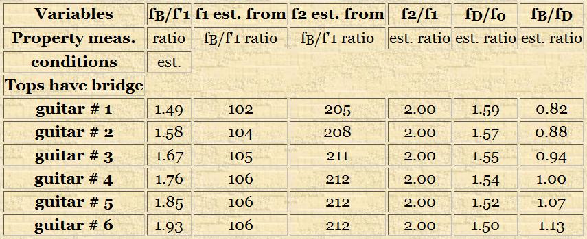
Part 2 — Reverse Modeling — Trying to copy an instrument with a particular set of final resonance ratios
Now let’s suppose that you’ve run across an instrument that sounds particularly fine to your ears and you’d like to understand more about what it is that made it behave like that. If you can make reasonable guesses as to what fO, f B and f D were during construction, and you have a general idea as to approximate bracing layout, top and back thickness’ and body dimensions, then you have a fighting chance of trying to re-create them.
Which of the Meyer variables can we measure in a finished instrument? By looking at Figure 6, we can see that f1 and f2 can be measured on the instrument with no particular alteration. That is, by muffling the strings, holding the neck halfway between the nut and where the neck joins the body and recording the tap tone from the center of the bridge, the air resonance and the first fundamental should be the two largest, low frequency peaks in the deconvolved spectrum.
If we repeat the process but this time constrain the back from vibrating, then the tap tone will yield f ‘1 and f ‘2 . If the back of the instrument you are measuring is very stiff, then according to Meyer’s experiments both sets of tap tones should give nearly identical values for the top frequency and air resonance.
The final Meyer variable measurement involves constraining both the front and back from vibrating and measuring the Helmholz frequency f O, as described at the top of the article. Note that there should be a progressive increase in the values of the air resonance as we increasingly constrain the front and back of the body.
Now what? Well, the only Meyer variables that we don’t know are f B and f D .
Equation (1) uses the ratio f D/fO to predict f ‘1/f O . The range of f D/f O shown by Meyer is about 0.6 – 1.6 (Figure 2) ; but more likely values are in the 1.4-1.6 range. We can easily set up a spreadsheet with the latter range of values and equation (1) and compare an estimated f ‘1/f O with the actual f ‘1/f O ratio created from the measurements we’ve just made. When we find a satisfactory value of the f D/fO ratio, we can solve for f D because we know f O .
Equation (2) also uses the ratio f D/fO , now to predict f ‘2/f O . Since the typical range of f D/f O is about 0.9 – 1.6 (Figure 3) we can set up another portion of the spreadsheet with this range of values and equation (2) and compare an estimated f ‘2/f O with the actual f ‘2/f O ratio created from the measurements we’ve just made. Once again, we can solve for f D because we know f O . A comparison of the two f D estimates will give us a sense of how accurate such predictions may be.
Equations (3) and (4) use the ratio f B/f ‘ 1 to predict f 2/f ‘2 and f 1/f ‘1 respectively. We can now use the same approach that we did for equations (1) and (2) to solve for f B . The name of the spreadsheet is MEYERCALCRVRS.XLS.
MEYERCALCRVRS (to download double-click or option-click)
At this point it would be useful to look at the spreadsheet so that we can walk our way through the calculations. The table below shows the values I’ve chosen for the spreadsheet as an exercise using guitar #6 in the forward modeling exercise above.
Table 3. Initial measured values for reverse modeling calculations 
When the worksheet is opened, the user will note two different colors: blue cells are for user input and green cells are values calculated as a result of user input. There are four groups of three columns of values. When the values in Table 3 or any others measured by the user are entered into the appropriate cells on the worksheet, four columns of “measured ratios” are created as the right-hand column in each group. In each case, the “measured ratio” is the value that is to be compared against the center column of each group. The center column is created by a range of either f D/fO ratios (groups 1 and 2) or f B/f O ratios (groups 3 and 4) which are in column 1 of each group (blue color).
Using the values in Table 3 and looking at the first calculation group, we see that the value of the measured f ‘1/f O is 0.877. This value remains constant the length of the column. We want to compare this ratio with the numbers in column 2 which were generated by using equation (1) and the ratios in column 1. It appears for this example that an f D/fO ratio between 1.52 and 1.58 gives an estimated f ‘1/f O which is nearly the same as 0.877 . So if
f D/fO = 1.52 – 1.58
Then,
f D = fO * (1.52 – 1.58) = 198 – 205 Hz
values only slightly larger than the actual f D of 195 Hz. The second calculation group gives an f D/fO ratio of 1.50 and a resultant value for f D of 195 Hz, right on the money. The second calculation group also seems more sensitive to estimating the f D/fO ratio. I have taken the liberty of including a fourth column to each group to perform these estimates.
The third and fourth calculation groups give f B/f ‘ 1 ratios of 1.90 – 2.05 and 1.75 – 2.05 respectively. These ranges are clearly less accurate than the first two groups, but the results are still quite usable. The third calculation group estimate of f B is 217 – 234 Hz while the fourth group estimate is 200 – 234 Hz. The actual value of f B for these sample calculations is 220 Hz.
The importance of these calculations is at least three-fold: first, we gain some sense of how the resonances change during the building stages and from one style of building to another; second, we see that there is some understandable relationship between the final resonances and those actually controllable by the builder; and third, I suggest that there is some hope for taking a great instrument and at least finding out a little bit more about it’s initial acoustic properties.
I enjoy writing these pages and hope that they are interesting and useful to the reader. I’ve stopped weaving/building at this time and still need to generate some income in order to continue to expand this website with more useful articles. If this page was helpful to you and you would like to make a $10.00 donation in order to have more pages like it, please use the donation button below. Thank you.
